getAnalysisResults(design, dataInput,...)Data Analysis for Trials with Interim Stages
Gernot Wassmer
January 14, 2026
Estimation and p-Values in Group Sequential Designs
Wassmer and Brannath (2025), Chaps. 4 and 9, Robertson et al. (2023), Robertson et al. (2025)
- p-values:
- stagewise \(p\)-values
- Cumulative \(p\)-values
- Final analysis adjusted (“exact”) \(p\)-values
- Repeated \(p\,\)-values
- Estimation:
- Unadjusted CIs
- Final analysis adjusted (“exact”) CIs based on stagewise ordering
- Repeated Confidence Intervals (RCIs)
- Point estimates
Exact p-values: Ordering of sample space
In a fixed-sample design, a \(p\)-value is defined as
\[p = P_{H_0}(Z \geq z)\;.\]
In a group sequential design, define overall \(p\)-value at the end of the trial through
\[p_\text{final} = P_{H_0}\left((Z^*_{\mathcal K}, {\mathcal K}) \succeq (z^*_k,k)\right)\;.\]
Needs ordering of the sample space
Focus on methods based on stagewise ordering of group-sequential sample space:
- Good theoretical properties
- Available in software (rpact, EaSt, etc.)
Example four-stage design, two-sided test
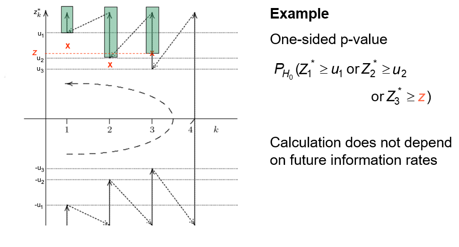
This \(p\)-value can only be calculated once, at the end of the trial
Overall repeated p-values
- The overall repeated \(p\,\)-value is the smallest significance level for which \(H_0\) can be rejected at stage \(k\) with the given data.
- Repeated \(p\,\)-values can be calculated at any stage of the trial.
- Repeated \(p\,\)-values exactly correspond to the test decision.
- Under \(H_0\), distribution of repeated \(p\,\)-value stochastically larger than uniform.
- Repeated \(p\,\)-values are conservative.
Confidence intervals and estimates
Confidence intervals:
- Repeated confidence intervals: sequence of intervals \(I_k\) for which
\[ P_\delta(\delta \in I_k \text{ for all } k = 1,\ldots,K) \geq 1 - \alpha \]
- Final analysis adjusted confidence interval, calculated by:
\[ P_{\delta^L}\left((Z^*_{\mathcal K}, {\mathcal K}) \succeq (z^*_k,k)\right) = \alpha/2 \text{ and } P_{\delta^U}\left((Z^*_{\mathcal K}, {\mathcal K}) \preceq (z^*_k,k)\right) = \alpha/2 \]
Point estimates:
Median unbiased estimator: Upper limit of a one-sided 50% confidence interval of the form \((-\infty; \delta_{0.5}]\).
Mid-point of RCI
Analysing a Trial with Interim Stages Using rpact
- Group sequential test
- Inverse normal combination test
- Fisher’s combination test
- Repeated confidence intervals, p-Values
- Final analysis adjusted confidence intervals, p-Values
- Conditional Rejection Probability (Müller & Schäfer)
- Conditional power assessment
- All this for continuous, binary, and survival endpoint
Group Sequential and Adaptive Analysis
design The trial design.
dataInput The summary data used for calculating the test results. This is either an element of DataSetMeans, of DataSetRates, or of DataSetSurvival.
Given a design and a dataset, at given stage the function calculates the test results (effect sizes, stage-wise test statistics and p-values, overall p-values and test statistics, conditional rejection probability (CRP), conditional power, Repeated Confidence Intervals (RCIs), repeated overall p-values, and final stage p-values, median unbiased effect estimates, and confidence intervals.)
The conditional power is calculated only if (at least) the sample size for the subsequent stage(s) is specified. Median unbiased effect estimates and confidence intervals are calculated only if a group sequential or an inverse normal design was chosen. A final stage \(p\)-value for Fisher’s combination test is calculated only if a two-stage design was chosen.
Group Sequential and Adaptive Analysis
dataInput
An element of
DataSetMeansfor one sample is created bygetDataset(means =, stDevs =, sampleSizes =)where
means, stDevs, sampleSizesare vectors with stagewise means, standard deviations, and sample sizes of length given by the number of available stages.
An element of
DataSetMeansfor two samples is created bygetDataset(means1 =, means2 =, stDevs1 =, stDevs2 =, sampleSizes1 =, sampleSizes2 =)where
means1, means2, stDevs1, stDevs2, sampleSizes1, sampleSizes2are vectors with stagewise means, standard deviations, and sample sizes for the two treatment groups of length given by the number of available stages.
Use of cumMeans, cumulativeMeans, overallMeans, cumStDevs, cumulativeStDevs, overallStDevs, n, cumN, etc., is also possible
Group Sequential and Adaptive Analysis
dataInput
An element of
DataSetMeansfor G + 1 samples is created bygetDataset(means1 =,..., means[G+1] =, stDevs1 =, ...,stDevs[G+1] =, sampleSizes1 =, ..., sampleSizes[G+1] =),where
means1, ..., means[G+1], stDevs1, ..., stDevs[G+1], sampleSizes1, ..., sampleSizes[G+1]are vectors with stagewise means, standard deviations, and sample sizes for G+1 treatment groups of length given by the number of available stages.Last treatment arm G + 1 always refers to the control group that cannot be deselected.
Only for the first stage all treatment arms needs to be specified, so treatment arm selection with an arbitrary number of treatment arms for subsequent stage can be considered.
Analogue definition of
DataSetRatesandDataSetSurvival: specifyevents.
Example Two-Sample Comparison of Rates
Define the design:
Wang and Tsiatis design with \(\Delta = 0.45\):
Data summary for binary data:
Analysis results
Analysis results for a binary endpoint
Sequential analysis with 4 looks (inverse normal combination test design), one-sided overall significance level 2.5%. The results were calculated using a two-sample test for rates, normal approximation test. H0: pi(1) - pi(2) = 0 against H1: pi(1) - pi(2) < 0.
| Stage | 1 | 2 | 3 | 4 |
|---|---|---|---|---|
| Fixed weight | 0.5 | 0.5 | 0.5 | 0.5 |
| Cumulative alpha spent | 0.0070 | 0.0138 | 0.0198 | 0.0250 |
| Stage levels (one-sided) | 0.0070 | 0.0088 | 0.0100 | 0.0110 |
| Efficacy boundary (z-value scale) | 2.456 | 2.372 | 2.325 | 2.291 |
| Cumulative effect size | -0.352 | -0.361 | -0.389 | |
| Cumulative treatment rate | 0.375 | 0.389 | 0.444 | |
| Cumulative control rate | 0.727 | 0.750 | 0.833 | |
| Stage-wise test statistic | -1.536 | -1.799 | -2.567 | |
| Stage-wise p-value | 0.0623 | 0.0360 | 0.0051 | |
| Inverse normal combination | 1.536 | 2.358 | 3.407 | |
| Test action | continue | continue | reject and stop | |
| Conditional rejection probability | 0.0777 | 0.3093 | 0.9062 | |
| 95% repeated confidence interval | [-0.739; 0.197] | [-0.646; 0.002] | [-0.618; -0.140] | |
| Repeated p-value | 0.1561 | 0.0259 | 0.0009 | |
| Final p-value | 0.0139 | |||
| Final confidence interval | [-0.598; -0.039] | |||
| Median unbiased estimate | -0.333 |
Check repeated p-value
Analysis results for a binary endpoint
Sequential analysis with 4 looks (inverse normal combination test design), one-sided overall significance level 2.59%. The results were calculated using a two-sample test for rates, normal approximation test. H0: pi(1) - pi(2) = 0 against H1: pi(1) - pi(2) < 0.
| Stage | 1 | 2 | 3 | 4 |
|---|---|---|---|---|
| Fixed weight | 0.5 | 0.5 | 0.5 | 0.5 |
| Cumulative alpha spent | 0.0073 | 0.0144 | 0.0205 | 0.0259 |
| Stage levels (one-sided) | 0.0073 | 0.0092 | 0.0104 | 0.0114 |
| Efficacy boundary (z-value scale) | 2.441 | 2.358 | 2.310 | 2.277 |
| Cumulative effect size | -0.352 | -0.361 | -0.389 | |
| Cumulative treatment rate | 0.375 | 0.389 | 0.444 | |
| Cumulative control rate | 0.727 | 0.750 | 0.833 | |
| Stage-wise test statistic | -1.536 | -1.799 | -2.567 | |
| Stage-wise p-value | 0.0623 | 0.0360 | 0.0051 | |
| Inverse normal combination | 1.536 | 2.358 | 3.407 | |
| Test action | continue | reject and stop | reject and stop | |
| Conditional rejection probability | 0.0806 | 0.3179 | 0.9109 | |
| 94.81% repeated confidence interval | [-0.737; 0.194] | [-0.644; 0.000] | [-0.617; -0.142] | |
| Repeated p-value | 0.1561 | 0.0259 | 0.0009 | |
| Final p-value | 0.0144 | |||
| Final confidence interval | [-0.656; -0.041] | |||
| Median unbiased estimate | -0.354 |
Check RCI
Analysis results for a binary endpoint
Sequential analysis with 4 looks (inverse normal combination test design), one-sided overall significance level 2.5%. The results were calculated using a two-sample test for rates, normal approximation test. H0: pi(1) - pi(2) = 0.0023 against H1: pi(1) - pi(2) < 0.0023.
| Stage | 1 | 2 | 3 | 4 |
|---|---|---|---|---|
| Fixed weight | 0.5 | 0.5 | 0.5 | 0.5 |
| Cumulative alpha spent | 0.0070 | 0.0138 | 0.0198 | 0.0250 |
| Stage levels (one-sided) | 0.0070 | 0.0088 | 0.0100 | 0.0110 |
| Efficacy boundary (z-value scale) | 2.456 | 2.372 | 2.325 | 2.291 |
| Cumulative effect size | -0.352 | -0.361 | -0.389 | |
| Cumulative treatment rate | 0.375 | 0.389 | 0.444 | |
| Cumulative control rate | 0.727 | 0.750 | 0.833 | |
| Stage-wise test statistic | -1.546 | -1.810 | -2.577 | |
| Stage-wise p-value | 0.0611 | 0.0352 | 0.0050 | |
| Inverse normal combination | 1.546 | 2.373 | 3.425 | |
| Test action | continue | reject and stop | reject and stop | |
| Conditional rejection probability | 0.0789 | 0.3163 | 0.9114 | |
| 95% repeated confidence interval | [-0.739; 0.197] | [-0.646; 0.002] | [-0.618; -0.140] | |
| Repeated p-value | 0.1536 | 0.0250 | 0.0008 | |
| Final p-value | 0.0138 | |||
| Final confidence interval | [-0.658; -0.039] | |||
| Median unbiased estimate | -0.354 |
Comparison of point estimates
[1] -0.3522727 -0.3611111 -0.3888889 NA[1] NA -0.3538987 NA NA[1] -0.2706451 -0.3216712 -0.3794755 NATesting means
Testing means
Analysis results for a continuous endpoint
Sequential analysis with 4 looks (inverse normal combination test design), one-sided overall significance level 2.5%. The results were calculated using a one-sample t-test. H0: mu = 0 against H1: mu > 0.
| Stage | 1 | 2 | 3 | 4 |
|---|---|---|---|---|
| Fixed weight | 0.5 | 0.5 | 0.5 | 0.5 |
| Cumulative alpha spent | 0.0070 | 0.0138 | 0.0198 | 0.0250 |
| Stage levels (one-sided) | 0.0070 | 0.0088 | 0.0100 | 0.0110 |
| Efficacy boundary (z-value scale) | 2.456 | 2.372 | 2.325 | 2.291 |
| Cumulative effect size | 0.330 | 0.383 | 0.379 | |
| Cumulative standard deviation | 0.970 | 0.941 | 0.918 | |
| Stage-wise test statistic | 1.800 | 2.856 | 2.264 | |
| Stage-wise p-value | 0.0415 | 0.0034 | 0.0157 | |
| Inverse normal combination | 1.733 | 3.138 | 3.804 | |
| Test action | continue | reject and stop | reject and stop | |
| Conditional rejection probability | 0.1040 | 0.7069 | 0.9776 | |
| 95% repeated confidence interval | [-0.151; 0.811] | [0.097; 0.662] | [0.152; 0.601] | |
| Repeated p-value | 0.1120 | 0.0028 | 0.0002 | |
| Final p-value | 0.0075 | |||
| Final confidence interval | [0.077; 0.577] | |||
| Median unbiased estimate | 0.342 |
Comparison of point estimates
Example Survival Analysis
Interim Analysis Stage
Suppose at the interim analysis, the observed number of events is 67 and the value of the (one-sided) Z-statistic is -1.10 (where negative values correspond to treatment benefit).
Re-calculate the stopping boundary based on the observed 67 events at the interim analysis.
- Assume the alpha-spending function is O’Brien and Fleming with a planned futility stop if one-sided \(p_1 \geq 0.5\).
- Assume the planned maximum number of events is 121.
What is the interim analysis decision?
Test decision
Continue to the next stage, since the Z statistic is between 0 (futility bound) and -2.795 (efficacy bound)
\(\hspace{1.5cm}\)
Direction of test statistic
NOTE: The function getDesignGroupSequential() doesn’t know which direction of Z statistic indicates treatment benefit. By default, the critical values are displayed assuming positive Z is beneficial.
Final Analysis Stage
Suppose at the final analysis, the observed number of events is 129 and the value of the Z-statistic is -2.00 (where negative values correspond to treatment benefit).
Re-calculate the stopping boundary based on the observed 67 events at interim and 129 events at the final analysis.
Since we have deviated from the planned maximum number of events (= 121), our actual alpha spent no longer follows the O’Brien-Fleming-type alpha-spending function. Use the argument typeOfDesign = "asUser" instead.
$alphaSpent
[1] 0.002594128 0.024999990Final test decision
Reject the null hypothesis since Z < -1.9764
Alternative
Use maxInformation and getAnalysisResults()
Alternative
Analysis results for a survival endpoint
Sequential analysis with 2 looks (group sequential design), one-sided overall significance level 2.5%. The results were calculated using a two-sample logrank test. H0: hazard ratio = 1 against H1: hazard ratio < 1.
| Stage | 1 | 2 |
|---|---|---|
| Planned information rate | 55.4% | 100% |
| Cumulative alpha spent | 0.0026 | 0.0250 |
| Stage levels (one-sided) | 0.0026 | 0.0242 |
| Efficacy boundary (z-value scale) | 2.795 | 1.974 |
| Cumulative effect size | 0.764 | |
| Overall test statistic | -1.100 | |
| Overall p-value | 0.1357 | |
| Test action | continue | |
| Conditional rejection probability | 0.0418 | |
| 95% repeated confidence interval | [0.386; 1.513] | |
| Repeated p-value | 0.2669 |
Second stage
Analysis results for a survival endpoint
Sequential analysis with 2 looks (group sequential design), one-sided overall significance level 2.5%. The results were calculated using a two-sample logrank test. H0: hazard ratio = 1 against H1: hazard ratio < 1.
| Stage | 1 | 2 |
|---|---|---|
| Planned information rate | 51.9% | 100% |
| Cumulative alpha spent | 0.0026 | 0.0250 |
| Stage levels (one-sided) | 0.0026 | 0.0241 |
| Efficacy boundary (z-value scale) | 2.795 | 1.976 |
| Cumulative effect size | 0.764 | 0.703 |
| Overall test statistic | -1.100 | -2.000 |
| Overall p-value | 0.1357 | 0.0228 |
| Test action | continue | reject |
| Conditional rejection probability | 0.0439 | |
| 95% repeated confidence interval | [0.386; 1.513] | [0.496; 0.996] |
| Repeated p-value | 0.2669 | |
| Final p-value | 0.0237 | |
| Final confidence interval | [0.498; 0.996] | |
| Median unbiased estimate | 0.704 |
Summary
- This way can only be performed with group sequential \(\alpha\)-spending function approach
- Best applicable for survival designs
- Note that number of stages need not to be fixed in advance
- Under-running can be taken into account using parameter
informationEpsilon - Examples see vignette An Example to Illustrate Boundary Re-Calculations during the Trial with rpact
References
Robertson, D. S., Thomas Burnett, Babak Choodari-Oskooei, Munya Dimairo, Michael Grayling, Philip Pallmann, and Thomas Jaki. 2025. “Confidence Intervals for Adaptive Trial Designs I: A Methodological Review.” Statistics in Medicine 44 (18-19): e70174.
Robertson, D. S., Babak Choodari-Oskooei, Munya Dimairo, Laura Flight, Philip Pallmann, and Thomas Jaki. 2023. “Point Estimation for Adaptive Trial Designs I: A Methodological Review.” Statistics in Medicine 42 (2): 122–45.
Wassmer, Gernot, and Werner Brannath. 2025. Group Sequential and Confirmatory Adaptive Designs in Clinical Trials. 2nd ed. Springer. https://link.springer.com/book/10.1007/978-3-031-89669-9.