getSampleSizeMeans(
    alternative = 10,
    stDev = 24,
    sided = 2,
    alpha = 0.05,
    beta = 0.2,
    allocationRatioPlanned = 2) |>
summary() Designing Trials with Different Types of Endpoints
Gernot Wassmer
January 14, 2026
Sample Size Calculation for Continuous Endpoint
Design without interim analyses
alternativeis the alternative hypothesis value. This can be a vector of assumed alternatives (default isseq(0.2, 1, 0.2))stDevis the standard deviation (default is 1). IfmeanRatio = TRUEis specified,stDevdefines the coefficient of variationsigma/mu2allocationRatioPlannedThe planned allocation ratio for a two treatment groups design (default is 1);
e.g.,allocationRatioPlanned = 2: 2(intervention) : 1(control)
IfallocationRatioPlanned = 0is entered, the optimal allocation ratio yielding the smallest overall sample size is determined
Design without interim analyses
Sample size calculation for a continuous endpoint
Fixed sample analysis, two-sided significance level 5%, power 80%. The results were calculated for a two-sample t-test, H0: mu(1) - mu(2) = 0, H1: effect = 10, standard deviation = 24, planned allocation ratio = 2.
| Stage | Fixed |
|---|---|
| Stage level (two-sided) | 0.0500 |
| Efficacy boundary (z-value scale) | 1.960 |
| Lower efficacy boundary (t) | -7.004 |
| Upper efficacy boundary (t) | 7.004 |
| Number of subjects | 205.4 |
Legend:
- (t): treatment effect scale
Design with interim analyses
(t) treatment effect scale: Minimal detectable difference (MDD), i.e., smallest difference in observed means that would lead to a rejection or futility stop at this stage (assuming observed standard deviation as specified.)
Design with interim analyses
Sample size calculation for a continuous endpoint
Sequential analysis with a maximum of 3 looks (group sequential design), one-sided overall significance level 2.5%, power 80%. The results were calculated for a two-sample t-test, H0: mu(1) - mu(2) = 0, H1: effect = 10, standard deviation = 24, planned allocation ratio = 2.
| Stage | 1 | 2 | 3 |
|---|---|---|---|
| Planned information rate | 30% | 60% | 100% |
| Cumulative alpha spent | <0.0001 | 0.0038 | 0.0250 |
| Stage levels (one-sided) | <0.0001 | 0.0038 | 0.0238 |
| Efficacy boundary (z-value scale) | 3.929 | 2.670 | 1.981 |
| Futility boundary (z-value scale) | 0 | -Inf | |
| Efficacy boundary (t) | 26.286 | 12.016 | 6.836 |
| Futility boundary (t) | 0 | ||
| Cumulative power | 0.0096 | 0.3359 | 0.8000 |
| Number of subjects | 66.0 | 132.1 | 220.1 |
| Expected number of subjects under H1 | 181.3 | ||
| Overall exit probability (under H0) | 0.5000 | 0.0038 | |
| Overall exit probability (under H1) | 0.0657 | 0.3262 | |
| Exit probability for efficacy (under H0) | <0.0001 | 0.0038 | |
| Exit probability for efficacy (under H1) | 0.0096 | 0.3262 | |
| Exit probability for futility (under H0) | 0.5000 | 0 | |
| Exit probability for futility (under H1) | 0.0561 | 0 |
Legend:
- (t): treatment effect scale
More on continuous endpoints
E.g., vignette Designing group-sequential trials with two groups and a continuous endpoint with rpact, written with Marcel Wolbers.
Also contains information on:
- Power calculations \(\rightarrow\)
getPowerMeans(maxNumberOfSubjects = ) - Sample size for non-inferiority trials
- Plotting designs
Sample Size Calculation for Binary Endpoint
Design without interim analyses
pi1andpi2are the assumed probabilities in the treatment (intervention) and control group if two treatment groups are considered,pi1is the alternative probability for a one treatment group design;pi1can be a vector, default isseq(0.4, 0.6, 0.1)allocationRatioPlannedis the planned allocation ratio for a two treatment groups design (default is 1).
IfallocationRatioPlanned = 0is entered, the optimal allocation ratio yielding the smallest overall sample size is determinedriskRatioIfriskRatio = TRUEis specified the sample size for one-sided testing of H0: pi1/pi2 = thetaH0 is calculated (default isFALSE)
Design without interim analyses
Sample size calculation for a binary endpoint
Fixed sample analysis, two-sided significance level 5%, power 80%. The results were calculated for a two-sample test for rates (normal approximation), H0: pi(1) - pi(2) = 0, H1: pi(1) = 0.4, control rate pi(2) = 0.25, optimum planned allocation ratio = 0.953.
| Stage | Fixed |
|---|---|
| Stage level (two-sided) | 0.0500 |
| Efficacy boundary (z-value scale) | 1.960 |
| Lower efficacy boundary (t) | -0.091 |
| Upper efficacy boundary (t) | 0.103 |
| Number of subjects | 303.6 |
Legend:
- (t): treatment effect scale
Design with interim analyses
# Group-sequential design with O'Brien and Fleming type
# alpha-spending and one interim at 60% information
getDesignGroupSequential(
    sided = 2,
    alpha = 0.05,
    beta = 0.2,
    informationRates = c(0.6, 1),
    typeOfDesign = "asOF") |>

# Sample size calculation
getSampleSizeRates(
    pi2 = 0.25,
    pi1 = 0.4) |>
summary()
(t) treatment effect scale: Minimal detectable difference (MDD), i.e., smallest difference in observed means that would lead to a rejection or futility stop at this stage (assuming observed control as specified.)
Design with interim analyses
Sample size calculation for a binary endpoint
Sequential analysis with a maximum of 2 looks (group sequential design), two-sided overall significance level 5%, power 80%. The results were calculated for a two-sample test for rates (normal approximation), H0: pi(1) - pi(2) = 0, H1: pi(1) = 0.4, control rate pi(2) = 0.25.
| Stage | 1 | 2 |
|---|---|---|
| Planned information rate | 60% | 100% |
| Cumulative alpha spent | 0.0076 | 0.0500 |
| Stage levels (two-sided) | 0.0076 | 0.0476 |
| Efficacy boundary (z-value scale) | 2.669 | 1.981 |
| Lower efficacy boundary (t) | -0.150 | -0.091 |
| Upper efficacy boundary (t) | 0.187 | 0.104 |
| Cumulative power | 0.3123 | 0.8000 |
| Number of subjects | 183.8 | 306.3 |
| Expected number of subjects under H1 | 268.1 | |
| Exit probability for efficacy (under H0) | 0.0076 | |
| Exit probability for efficacy (under H1) | 0.3123 |
Legend:
- (t): treatment effect scale
More on binary endpoints
vignette Planning a trial with binary endpoints with rpact.
- Power calculations \(\rightarrow\)
getPowerRates(maxNumberOfSubjects = ) - Sample size for non-inferiority trials
- Sample size for single arm trials
- Plotting designs
Survival Design
We assume:
- \(\alpha = 0.025\)
- \(\pi_1 = 0.229\), \(\pi_2 = 0.37\) at 6 months
- Power \(1 - \beta = 0.85\) at \(\omega = \frac{\ln(1 - \pi_1)}{\ln(1 - \pi_2)} = 0.563\)
- Allocation ratio 1 : 1
We wish to test
\(H_0: \omega \geq 1 \text{ against } H_1: \omega < 1\)
rpact planning
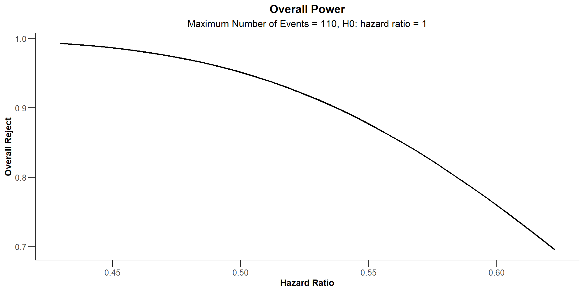
Start with fixed sample size (events) design:
Sample size calculation for a survival endpoint
Fixed sample analysis, one-sided significance level 2.5%, power 85%. The results were calculated for a two-sample logrank test, H0: hazard ratio = 1, H1: hazard ratio = 0.563, control pi(2) = 0.2, event time = 12, accrual time = 12, accrual intensity = 57.4, follow-up time = 6.
| Stage | Fixed |
|---|---|
| Stage level (one-sided) | 0.0250 |
| Efficacy boundary (z-value scale) | 1.960 |
| Efficacy boundary (t) | 0.687 |
| Number of subjects | 689.1 |
| Number of events | 108.8 |
| Analysis time | 18.00 |
| Expected study duration under H1 | 18.00 |
Legend:
- (t): treatment effect scale
Required Number Of Events
109 events are needed to achieve 85% power for specified effect size
Required Number Of Subjects
Obviously, some default parameters were used to derive the required number of subjects
Design plan parameters and output for survival data
Design parameters
- Critical values: 1.960
- Significance level: 0.0250
- Type II error rate: 0.1500
- Test: one-sided
User defined parameters
- Hazard ratio: 0.563
Default parameters
- Theta H0: 1
- Type of computation: Schoenfeld
- Assumed control rate: 0.200
- Planned allocation ratio: 1
- Event time: 12
- Accrual time: 12.00
- kappa: 1
- Follow up time: 6.00
- Drop-out rate (1): 0.000
- Drop-out rate (2): 0.000
- Drop-out time: 12.00
Sample size and output
- Direction upper: FALSE
- Assumed treatment rate: 0.118
- median(1): 66.2
- median(2): 37.3
- lambda(1): 0.0105
- lambda(2): 0.0186
- Number of events: 108.8
- Accrual intensity: 57.4
- Number of events fixed: 108.8
- Number of subjects fixed: 689.1
- Number of subjects fixed (1): 344.6
- Number of subjects fixed (2): 344.6
- Analysis time: 18.00
- Study duration: 18.00
- Critical values (treatment effect scale): 0.687
Legend
- (i): values of treatment arm i
Study specifications
- accrual time = 24
- study duration = 28
- drop-out rate = 0.25 at 6 months
- planned number of participants = 325
Study specifications
Sample size calculation for a survival endpoint
Fixed sample analysis, one-sided significance level 2.5%, power 85%. The results were calculated for a two-sample logrank test, H0: hazard ratio = 1, H1: treatment pi(1) = 0.229, control pi(2) = 0.37, event time = 6, accrual time = 24, accrual intensity = 10.8, follow-up time = 4, dropout rate(1) = 0.25, dropout rate(2) = 0.25, dropout time = 6.
| Stage | Fixed |
|---|---|
| Stage level (one-sided) | 0.0250 |
| Efficacy boundary (z-value scale) | 1.960 |
| Efficacy boundary (t) | 0.687 |
| Number of subjects | 259.2 |
| Number of events | 108.7 |
| Analysis time | 28.00 |
| Expected study duration under H1 | 28.00 |
Legend:
- (t): treatment effect scale
Follow-up time can be reduced with 325 participants:
Follow-up time can be reduced with 325 participants:
Sample size calculation for a survival endpoint
Fixed sample analysis, one-sided significance level 2.5%, power 85%. The results were calculated for a two-sample logrank test, H0: hazard ratio = 1, H1: treatment pi(1) = 0.229, control pi(2) = 0.37, number of subjects = 325, event time = 6, accrual time = 24, accrual intensity = 13.5, dropout rate(1) = 0.25, dropout rate(2) = 0.25, dropout time = 6.
| Stage | Fixed |
|---|---|
| Stage level (one-sided) | 0.0250 |
| Efficacy boundary (z-value scale) | 1.960 |
| Efficacy boundary (t) | 0.687 |
| Number of subjects | 325.0 |
| Number of events | 108.7 |
| Analysis time | 23.18 |
| Expected study duration under H1 | 23.18 |
Legend:
- (t): treatment effect scale
Design with interim stage
designGS <- getDesignGroupSequential(
    directionUpper = FALSE,
    alpha = 0.025,
    beta = 0.15,
    typeOfDesign = "asHSD",
    gammaA = -4.5,
    informationRates = c(2/3, 1)
)
getSampleSizeSurvival(
    design = designGS,
    pi1 = 0.229,
    pi2 = 0.37,
    eventTime = 6,
    accrualTime = 24,
    followUpTime = 4,
    dropoutRate1 = 0.25,
    dropoutRate2 = 0.25,
    dropoutTime = 6
) |> summary()
Design with interim stage
Sample size calculation for a survival endpoint
Sequential analysis with a maximum of 2 looks (group sequential design), one-sided overall significance level 2.5%, power 85%. The results were calculated for a two-sample logrank test, H0: hazard ratio = 1, H1: treatment pi(1) = 0.229, control pi(2) = 0.37, event time = 6, accrual time = 24, accrual intensity = 10.9, follow-up time = 4, dropout rate(1) = 0.25, dropout rate(2) = 0.25, dropout time = 6.
| Stage | 1 | 2 |
|---|---|---|
| Planned information rate | 66.7% | 100% |
| Cumulative alpha spent | 0.0054 | 0.0250 |
| Stage levels (one-sided) | 0.0054 | 0.0235 |
| Efficacy boundary (z-value scale) | 2.552 | 1.987 |
| Efficacy boundary (t) | 0.551 | 0.684 |
| Cumulative power | 0.4629 | 0.8500 |
| Number of subjects | 223.7 | 261.8 |
| Expected number of subjects under H1 | 244.1 | |
| Cumulative number of events | 73.2 | 109.8 |
| Expected number of events under H1 | 92.9 | |
| Analysis time | 20.51 | 28.00 |
| Expected study duration under H1 | 24.53 | |
| Exit probability for efficacy (under H0) | 0.0054 | |
| Exit probability for efficacy (under H1) | 0.4629 |
Legend:
- (t): treatment effect scale
Results
110 events are needed to achieve 85% power
262 study participants are needed to expect required number of events at given accrual and follow-up
drop-outs taken into account
325 planned participants are expected to achieve study goal in a shorter time frame
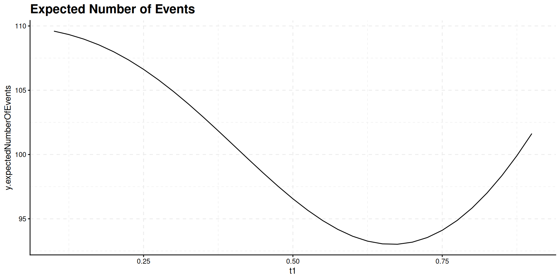
When should the interim take place?
library(ggplot2)
library(ggpubr) # This for the grids

infRates <- seq(0.1, 0.9, 0.05)
power <- Vectorize(function(x) {
    getDesignGroupSequential(
        directionUpper = FALSE,
        alpha = 0.025,
        typeOfDesign = "asHSD",
        gammaA = -4.5,
        informationRates = c(x, 1)
    ) |>
    getPowerSurvival(
        hazardRatio = 0.563,
        pi2 = 0.37,
        eventTime = 6,
        maxNumberOfEvents = 110,
        maxNumberOfSubjects = 262,
        accrualTime = 24
    ) |> fetch(overallReject)
})
ggplot(data.frame(infRates = infRates, power = power(infRates)),
       aes(infRates, power)
      ) +
  geom_line() + ylim(0.83, 0.87) +
  geom_hline(yintercept = 0.85, linetype = 2, lwd = 0.5, color = "red") +
  ggtitle("Overall Power") +
  theme_classic() + grids(linetype = "dashed") +
  theme(plot.title=element_text(face='bold', size=16))
When should the interim take place?
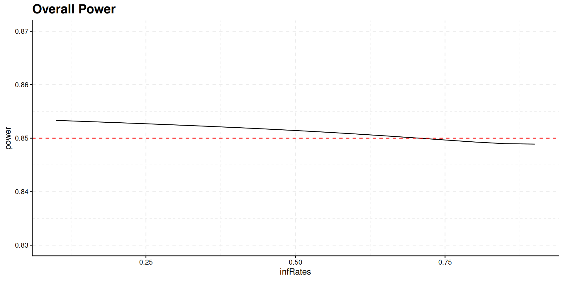
Interim time point has negligible influence on power but has effect on expected study duration, i.e., on expected number of events:

Summary
- For survival designs, many additional options for specifying patient recruitment, survival time distribution, and effect size pattern available, see vignette Planning a Survival Trial with rpact
- Flexible trial conduct through use of \(\alpha\)-spending approach
- Caveat: No data-driven reassessment of information possible without jeopardizing Type I error control
- Alternative: p-value combination approach: use of inverse normal combination of Fisher’s combination test
- Application, e.g., within promizing zone design, see vignette Promizing Zone Design with rpact
- Use of fast and flexible
getSimulationSurvival()function for assessing these designs