Design Specification in rpact

Gernot Wassmer

RPACT

January 14, 2026

Work-flow for sample size calculations in rpact

Define abstract group-sequential boundaries which are applicable to any type of endpoint (getDesignGroupSequential()).
Feed these boundaries into endpoint-specific sample size formulas (e.g., getSampleSizeMeans(), getSampleSizeRates(), getSampleSizeSurvival(), getSimulationxxx(), getPowerxxx()).
For trials without interim analyses, Step 1. can be omitted.
getDesignInverseNormal() yields the same results as getDesignGroupSequential(), it has an effect only for simulation and analysis.
getDesignFisher() provides no planning calculation, use the simulation tools instead.

Abstract group-sequential boundaries

Function getDesignGroupSequential() derives group-sequential boundaries in the mathematically simplest case:

Single arm trial with independent \(X_i \sim N(\mu,1)\)
Test \(H_0: \mu = 0\) against \(H_1: \mu = 1\)
Correlation structure between \(Z\)-statistics at interim and final analyses is identical for more complex situations (e.g., binary, continuous and survival endpoints).

Group-sequential boundaries and properties of the design apply to all endpoints!

Example: O’Brien-Fleming type \(\alpha\)-spending

design <- getDesignGroupSequential(
    sided = 2, 
    alpha = 0.05, 
    beta = 0.2,
    informationRates = c(0.3, 0.6, 1),
    typeOfDesign = "asOF")

informationRates: information fractions at which interim and final analysis are conducted.
Information fraction \(t_k\) at analysis \(k\):
- Binary and normal outcomes: \(t_k = n_k/N_{max}\)
- Survival outcomes: \(t_k = d_k/d_{max}\) where d is # events.
typeOfDesign = "asOF": O’Brien and Fleming type \(\alpha\)-spending.

Supported efficacy boundaries

Argument typeOfDesign:

Exact O’Brien & Fleming (“OF”), Pocock (“P”), Wang and Tsiatis (“WT”), Haybittle and Peto (“HP”)
Pampallona and Tsiatis (“PT”) one-sided and two-sided designs
O’Brien & Fleming and Pocock type \(\alpha\)-spending (“asOF” and “asP”)
Kim & DeMets (“asKD”) and Hwang, Shi and DeCani \(\alpha\)-spending (“asHSD”) and \(\beta\)-spending (“bsKD” and (“bsHSD”))
User-defined \(\alpha\)-spending (“asUser”) and \(\beta\)-spending (“bsUser”)
No early efficacy stops (“noEarlyEfficacy”)

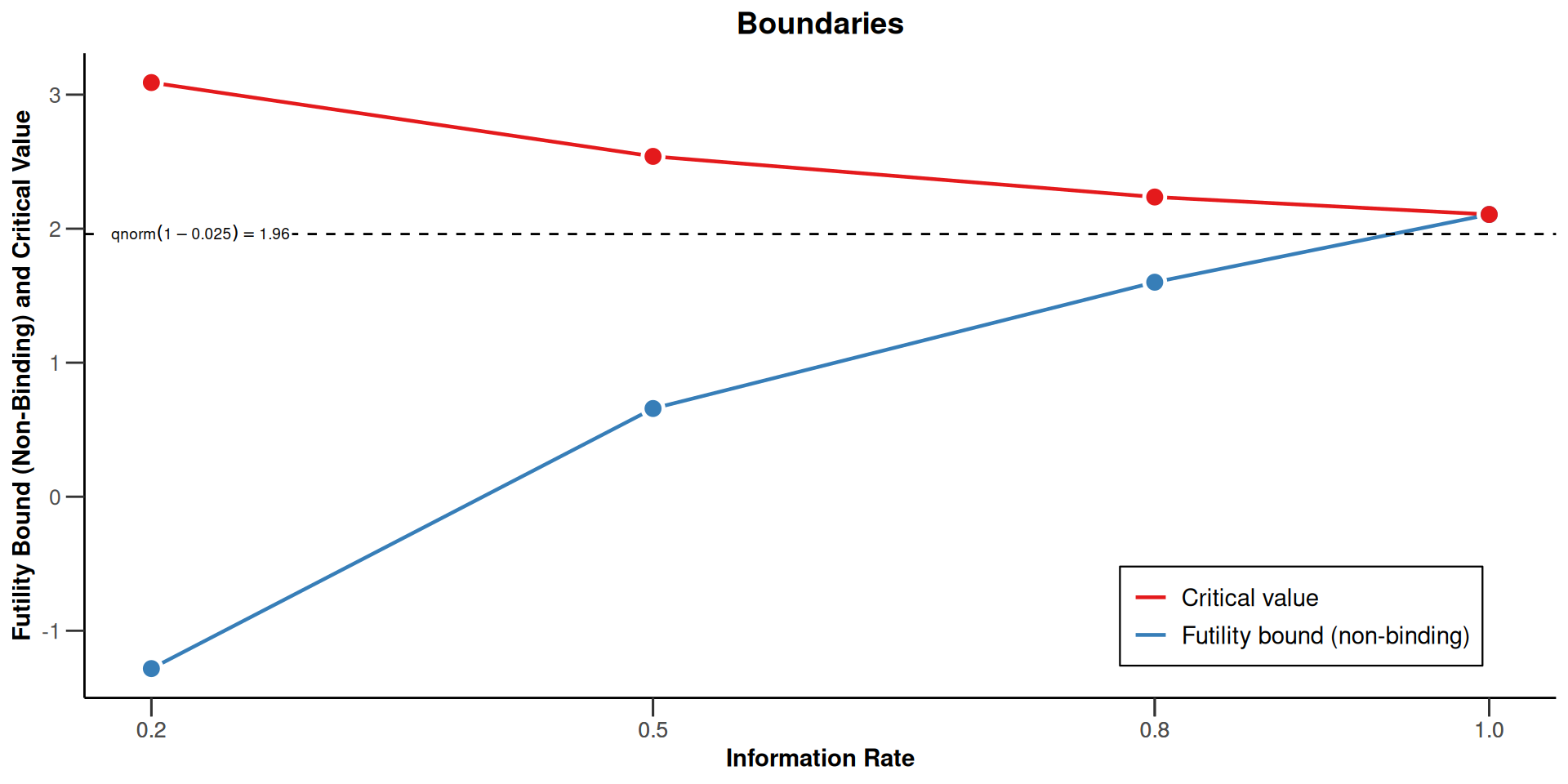
Example: Futility boundaries

# Example: non-binding futility boundary at first interim in
# case estimated treatment effect is null or in "the wrong
# direction", no futility at second interim
design <- getDesignGroupSequential(
    sided = 1, 
    alpha = 0.025, 
    beta = 0.2,
    informationRates = c(0.3, 0.6, 1),
    typeOfDesign = "asOF",
    futilityBounds = c(0, -Inf),
    bindingFutility = FALSE) 
summary(design)

futilityBounds: Vector on \(z\)-value scale for interim analyses (excluding final analysis).
z = 0: Futility if “null effect or effect in wrong direction”
z = -Inf: No futility at this interim analysis
bindingFutility = FALSE (default): no effect on efficacy boundaries.
futilityBounds only supported for one-sided testing.

Example: Futility boundaries

Sequential analysis with a maximum of 3 looks (group sequential design)

O’Brien & Fleming type alpha spending design, non-binding futility, one-sided overall significance level 2.5%, power 80%, undefined endpoint, inflation factor 1.0718, ASN H1 0.8826, ASN H01 0.8852, ASN H0 0.695.

Stage	1	2	3
Planned information rate	30%	60%	100%
Cumulative alpha spent	<0.0001	0.0038	0.0250
Stage levels (one-sided)	<0.0001	0.0038	0.0238
Efficacy boundary (z-value scale)	3.929	2.670	1.981
Futility boundary (z-value scale)	0	-Inf
Cumulative power	0.0096	0.3359	0.8000
Futility probabilities under H1	0.056	0

Additional characteristics of the design

getDesignCharacteristics(design)

Group sequential design characteristics

Number of subjects fixed: 7.8489
Shift: 8.4123
Inflation factor: 1.0718
Informations: 2.524, 5.047, 8.412
Power: 0.009643, 0.335884, 0.800000
Rejection probabilities under H1: 0.009643, 0.326241, 0.464116
Futility probabilities under H1: 0.05607, 0
Ratio expected vs fixed sample size under H1: 0.8826
Ratio expected vs fixed sample size under a value between H0 and H1: 0.8852
Ratio expected vs fixed sample size under H0: 0.6950

Number of subjects fixed: for abstract design without interim analyses.
Shift: Maximal sample size for abstract design with interim analyses.
Inflaction factor: Maximum sample size increase of sequential design relative to design without interim analyses.
Ratio expected vs fixed sample size: Reduction in expected sample size of sequential relative to fixed design.

Stopping probabilities under \(H_0\) and \(H_1\)

nMax <- getDesignCharacteristics(design)$shift

getPowerAndAverageSampleNumber(
    design,
    theta = 0, 
    nMax = nMax)

Power and average sample size (ASN)

User defined parameters

N_max: 8.4123
Effect: 0

Output

Average sample sizes (ASN): 5.455
Power: 0.02344
Early stop: 0.5038
Early stop [1]: 0.500043
Early stop [2]: 0.003758
Early stop [3]: NA
Overall reject: 0.02344
Reject per stage [1]: 4.273e-05
Reject per stage [2]: 0.003758
Reject per stage [3]: 0.01964
Overall futility: 0.5000
Futility stop per stage [1]: 0.5000
Futility stop per stage [2]: 0.0000

Legend

[k]: values at stage k

nMax <- getDesignCharacteristics(design)$shift

getPowerAndAverageSampleNumber(
    design,
    theta = 1, 
    nMax = nMax)

Power and average sample size (ASN)

User defined parameters

N_max: 8.4123
Effect: 1

Output

Average sample sizes (ASN): 6.928
Power: 0.8000
Early stop: 0.3920
Early stop [1]: 0.06572
Early stop [2]: 0.32624
Early stop [3]: NA
Overall reject: 0.8000
Reject per stage [1]: 0.009643
Reject per stage [2]: 0.326241
Reject per stage [3]: 0.464116
Overall futility: 0.05607
Futility stop per stage [1]: 0.05607
Futility stop per stage [2]: 0.00000

Legend

[k]: values at stage k

Example: Derivation of futility bounds

design <- getDesignInverseNormal(
    kMax = 4, 
    alpha = 0.025,
    typeOfDesign = "asKD", 
    gammaA = 2,
    informationRates = c(0.2, 0.5, 0.8, 1),
    typeBetaSpending = "bsOF", 
    beta = 0.2,
    bindingFutility = FALSE)
plot(design, type = 1)

Design Specification in rpact

Work-flow for sample size calculations in rpact

Abstract group-sequential boundaries

Example: O’Brien-Fleming type \(\alpha\)-spending

Supported efficacy boundaries

Example: Futility boundaries

Example: Futility boundaries

Additional characteristics of the design

Stopping probabilities under \(H_0\) and \(H_1\)

Example: Derivation of futility bounds

More on group-sequential boundaries